


Graph-Data Structure


Overview
Graphs provide the ultimate in data structure flexibility. A graph consists of a set of nodes, and a set of edges where an edge connects two nodes. Trees and lists can be viewed as special cases of graphs. And the core graph algorithms including traversal, topological sort, shortest paths algorithms, and algorithms to find the minimal-cost spanning tree.
A graph can be represent as
It consists of a set of vertices(Another name for a node in a graph) V and a set of edges E, such that each edge in E is a connection between a pair of vertices in V. 1 the number of vertices is written |V|, and the number of edges is written |E|. |E| can range from zero to a maximum of |V|^2-|V|.
Note: All the illustrations are from the Credit section(bottom).
The Term of Concepts
These concepts below should be remembered.
Undirected, Directed and Labeled Graph
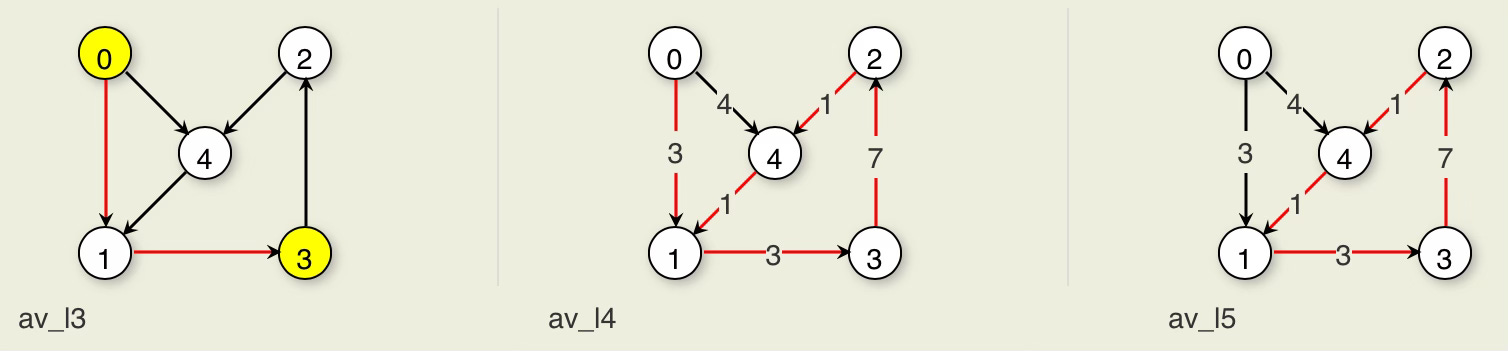
A graph whose edges are not directed is called an undirected graph, as shown in (a) of the following figure. A graph with edges directed from one vertex to another (as in (b)) is called a directed graph or digraph. A graph with labels associated with its vertices (as in (c)) is called a labeled graph. Associated with each edge may be a cost or weight. A graph whose edges have weights (as in (c)) is said to be a weighted graph.

Undirected Graph
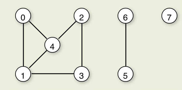
An undirected graph is a connected graph if there is at least one path form any vertex to any other. The maximally connected subgraphs of an undirected graph are called connected components. For example, this figure shows an undirected graph with three connected components.
Incident, Adjacent and Degree
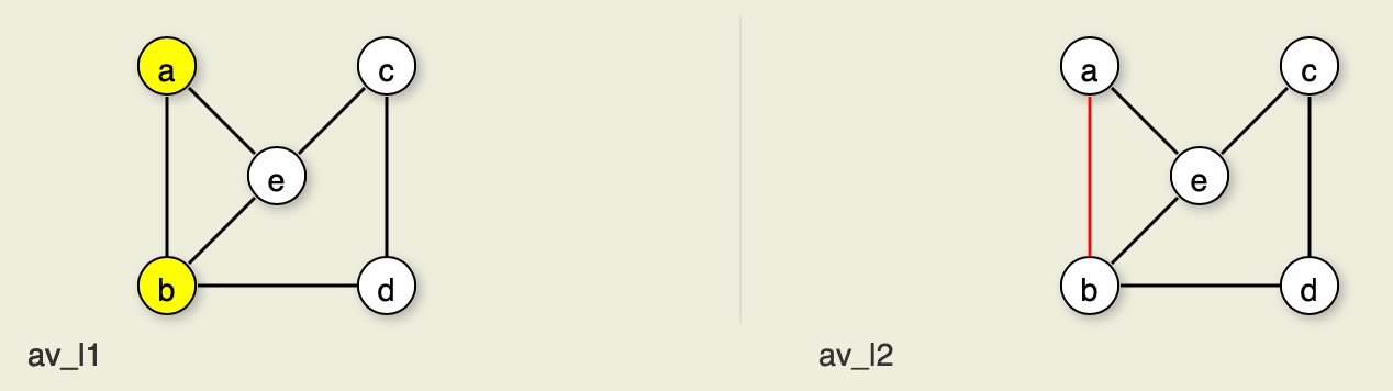
An edge connecting Vertices a and b is written (a,b). Such an edge is said to be incident the Vertices a and b. The two vertices are said to be adjacent. If the edge is directed from a to b, then we say that a is adjacent to b, and b is adjacent from a. The degree of a vertex is the number of edges it is incident with. For example, Vertex e below has a degree of three.
In a directed graph, the out degree for a vertex is the number of neighbours adjacent from it (or the number of edges coming in to it). In (c) above, the in degree of Vertex is two, and its out degree is one.
Simple Path and Cycle
A sequence of vertices v1,v2 …,vn forms a path of length n-1 if there exist edges from v1 to vi+1 for 1<=i<=n. A path is a simple path if all vertices on the path are distinct. The length of a path is the number of edges it contains. A cycle is a path of length three or more that connects some vertex v1 to itself. A cycle is a simple cycle if the path is simple, except for the first and last vertices being the same.
Sparse and Dense Graph
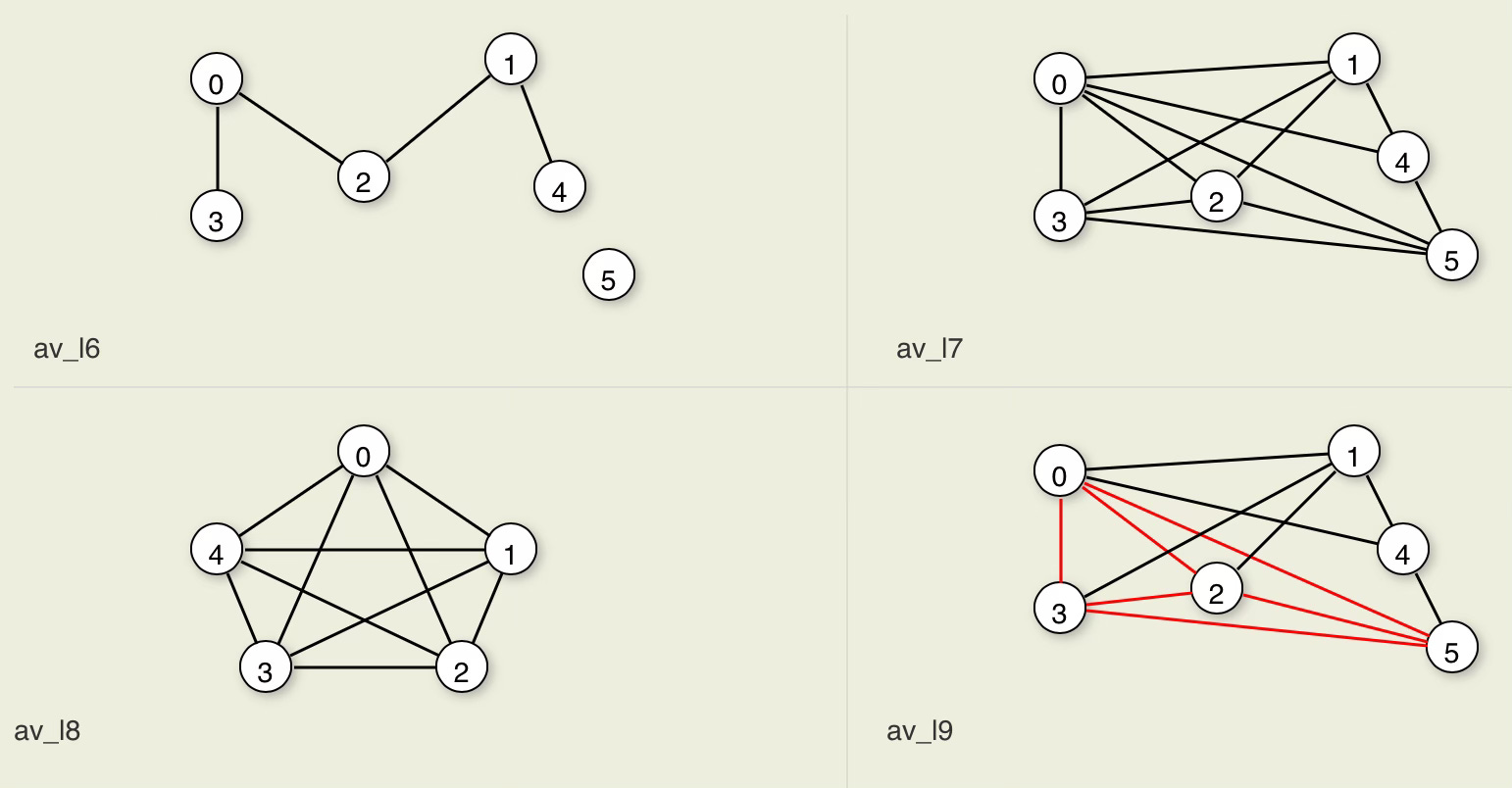
A graph with relatively few edges is called a sparse graph, while a graph with many edges is called a dense graph. A graph containing all possible edges is said to be a complete graph. A subgraph S is formed from graph G by selecting a subset Vs of G’s vertices and a subset Es of G’s edges such that for every edge:
And both vertices of e are in Vs. Any subgraph of V where all vertices in the graph connect to all other vertices in the subgraph is called a clique.
(Directed) Acyclic Graph
A graph without cycles is called an acyclic graph. Thus, directed graph without cycles is called a directed acyclic graph or DAG.
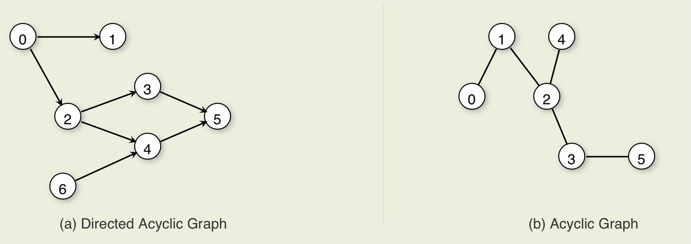
A free tree is a connected, undirected graph with no simple cycles. An equivalent definition is that a free tree is connected and has |V|-1 edges.
Graph Representations
There are two commonly used methods for representing graphs.
Adjacency Matrix
The adjacency matrix for a graph is a |V|x|V| array. We typically label the vertices from V0 through V|v|-1. Row i of the adjacency matrix contains entries for Vertex Vi. Column j in row I is marked if there is an edge from Vi to Vj and is not marked otherwise. The space requirements for the adjacency matrix are
Adjacency List
It is an array of linked lists. The array is |V| items long, with position i storing a pointer to the linked list of edges for Vertex Vi. This linked list represents the edges by the vertices that are adjacent to Vertex Vi.
Here is an example of two representations on a directed graph. The entry for Vertex 0 stores 1 and 4 because there are two edges in the graph leaving Vertex 0, with one going to Vertex 1 and one going to Vertex 4. The list for Vertex 2 stores an entry for Vertex 4 because there is an edge from Vertex 2 to Vertex 4, but no entry for Vertex 3 because this edge comes into Vertex 2 rather than going out.
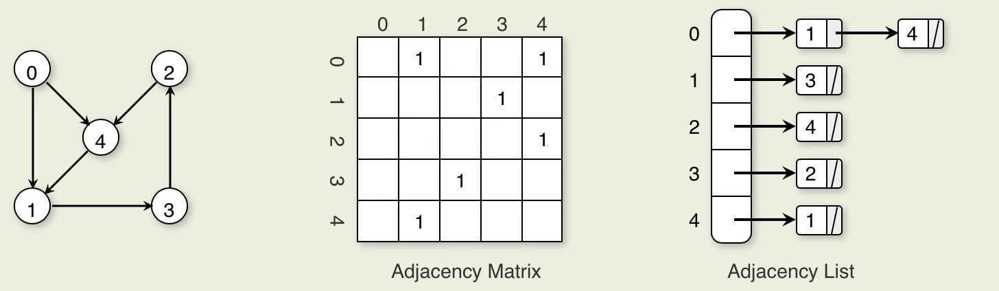
Representing a Directed Graph
Both the adjacency matrix and the adjacency list can be used to store directed or undirected graphs. Each edge of an undirected graph connecting Vertices u and v is represented by two directed edges: one from u to v and one from v to u. Here is an example of the two representations on an undirected graph. We see that there are twice as many edge entries in both the adjacency matrix and the adjacency list. For example, for the undirected graph, the list for Vertex 2 stores and entry for both Vertex3 and Vertex 4.
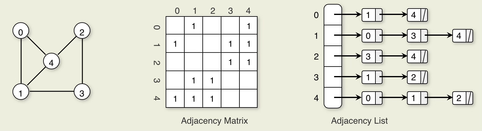
Representing an Undirected Graph
The storage requirements for the adjacency list depend on both the number of edges and the number of vertices in the graph. There must be an array entry for each vertex(even if the vertex is not adjacent to any other vertex and thus has no elements on its linked list), and each edge must appear on one for the lists. Thus, the cost is:
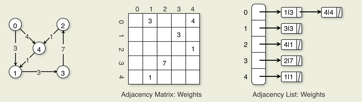
Sometimes we want to store weights or distances with each edge. This is easy with the adjacency matrix, where we will just store values for the weight in the matrix. For example, we store a value of “1“ at each position just ti show that the edge exists. That could have been done using a single bit, but since bit manipulation is typically complicated in most programming languages, an implementation might store a byte or an integer at each matrix position. For a weighted graph, we should need to store at each position in the matrix enough space to represent the weight, which might typically be an integer.
The adjacency list needs to explicitly store a weight with each edge. In the adjacency list shown below, each linked list node is shown storing two values. The first is the index for the neighbor at the end of the associated edge. The second is the value for the weight. As with the adjacency matrix, this value requires space to represent, typically an integer.
Conclusion
We talks about the terms concepts of Graph. This is the first step for entering the Deep learning. For example, we use PyTorch creating the graph and executing it. We will talk about this in next article.
Credit
https://opendsa-server.cs.vt.edu/ODSA/Books/bghs-stem-code-bcs/bcs2/spring-2020/1/html/GraphIntro.html#id2
https://arxiv.org/pdf/1610.08189.pdf